Quality by Design modelling for rapid RNA vaccine production

Below is the Documentation.md file to support the code of the following publication about Quality by design modelling to support rapid RNA vaccine production against emerging infectious diseases . It can be found here

Code by:

• Damien van de Berg
• Dr. Zoltán Kis

Manuscript co-authored by:

• Carl Fredrik Behmer
• Karnyart Samnuan
• Dr. Anna K. Blakney
• Dr. Cleo Kontoravdi
• Prof. Robin Shattock
• Prof. Nilay Shah

Background

This model aims to link effective RNA yield in RNA vaccine transcription, which is a grouped term representing the absolute RNA yield crtical quality attribute (CQA) minus degradation CQA. It is assumed that this effective RNA yield corresponds to a subset of the experimental RNA yield from a statistical Design Of Experiments dataset (cf. Experimental_Data.xlsx), namely a measurement of the mass of RNA sequences that are not degraded (have a certain minimum length).

Whereas the proposed CQA accounts for the necessary quantity of RNA produced, this does not account for other CQAs:

• Sequence identity is crucial in assuring translation of the RNA in the patient’s cell into the polypeptides that act as ‘active pharmaceutical ingredient’, and are recognised by the patient’s immune system as antigen.
• 5’capping: 5’capping of the RNA sequence not only protects the RNA from being degraded. In the patient’s cell, incorrect 5’capping can lead to the RNA sequence being recognised as foreign shutting down translation of RNA.

A lack of mechanistic, biological understanding is currently inhibiting the development of models that link sequence identity and 5’capping to critical process parameters (CPPs) such as spermidine concentration, and we want to refrain from using statistical or data-driven models in this manuscript.

We propose a simple mechanistic model linking the production of effective RNA yield (RNA yield CQA and degradation CQA) to the following critical process parameters:

• Reaction time
• Total initial Mg concentration
• Total initial NTP concentration
• Initial total T7RNAP enzyme concentration

Model

The buffer solution of the RNA transcription reactor is complex. It is assumed that the main species present in solution affecting transcription and degradtion kinetics are: Mg²⁺, NTP^4- (all nucleotides are assumed to be the same), H⁺, HEPES^- (buffer) and PPi^4- (pyrophosphate)

These 5 free solution components can form the following 10 complexes: HNTP^3-, MgNTP^2-, Mg₂NTP, MgHNTP^-, MgPPi²⁺, Mg₂PPi, HPPi^3-, H₂PPi^2-, MgHPPi^-

We propose the following system of differential-algebraic equations to model the RNA yield [𝑅𝑁𝐴]_𝑡𝑜𝑡 respresenting the CQA. In its differential expression, it can be seen that the production and consumption of [𝑅𝑁𝐴]_𝑡𝑜𝑡 consists of transcription and degradation kinetics as stand-ins for the respective CQAs.

Differential Expressions:

Kinetic Expressions:

Mass Balance Constraints:

Equilibrium Constraints:

The overall structure of the system, with differential equations describing the change in total concentrations and mass balance and equilibrium considerations giving the (free) solution concentrations that appear in the differential expressions was based on Akama et al.. The Michaelis-Menten term was also adapted from this paper. The degradation term was inspired by Li and Breaker and Bernhardt and Tate.

This gives a well-posed mathematical problem which can be solved using DAE solvers or in this case, using initial value differential ODE solvers to solve for the total concentrations, where at each time step the solution concentrations are obtained using algebraic solvers.

If possible, exisitng knowledge should be used as much as possible to determine the parameters of this model. As such, N_all is fixed to 10,000 as it represents the length of the nucleotide chain. Similarly, the equilibrium constants 𝐾_𝑒𝑞,0 to 𝐾_𝑒𝑞,8 were all listed in this publication: 𝐾_𝑒𝑞,0 = 10^-6.95, 𝐾_𝑒𝑞,1 = 10^-4.42, 𝐾_𝑒𝑞,2 = 10^-1.69, 𝐾_𝑒𝑞,3 = 10^-1.49, 𝐾_𝑒𝑞,4 = 10^-5.42, 𝐾_𝑒𝑞,5 = 10^-2.33, 𝐾_𝑒𝑞,6 = 10^-8.94, 𝐾_𝑒𝑞,7 = 10^-6.13, 𝐾_𝑒𝑞,8 = 10^-3.05 and 𝐾_eq,9 was taken to be 10^-7.5 (the K_A for HEPES buffer), all in M.

Model implementation

Python was chosen for this endeavor due to its accessability, and easy integration with data-driven methods in later stages of process development with established libraries (scikit-learn, …)

At first, canned ODE solvers such as scipy.integrate.odeint were used to solve the differential expressions (Eq. 1) to (Eq. 7). (Eq. 7) was omitted as total HEPES concentration should remain the same, as none is supposed to be converted or precipitate. However, it was found that the main bottleneck in the solution of this system was the robust determination of solution concentrations from total concentrations (M1 to M5 and E1 to E10). In fact, fsolve was very sensitive to the inital guesses provided, which were not known a priori and could be off by orders of magnitude.

Hence, at each time iteraton, instead of solving this whole algebraic system of 15 equations, a reduced system of 5 equations and only the 5 free solution concentrations was solved, obtained by substituting the expressions of (E1 to E10) into (M1-M5). For the initial conditions, an initial guess was searched that would give physical (non-negative) solutions. This search consisted in starting with the total concentration of the free solution concentrations as initial guesses, as this would usually be within an order of magnitude of the real solution. If this did not converge, the initial guesses were multiplied by a constant factor, until the initial guesses did converge.

To avoid this search for the initial guesses at each timestep, the solution to the free solution concentration system of one time step, would be the initial guess to the solver of the next step. This would most of the time be sufficient to find a physical solution, leading to significant computational savings. However, for the cases that it didn’t give non-negative solutions, the same search as for a valid initial guess was performed.

The main reason why an in-house implementation of Runge-Kutta is used as ODE solver, is because canned solvers (ODE 45 or similar) only return the independent and dependent variables of the differential system being solved. However, in future iterations, a time delay for Mg₂PPi precipitation might need to be considered. So with the in-house implementation, it is easier to return arguments different to solution concentrations from the ODE solver, such as initial guesses to the next timestep and precipitation time delays. Switching to canned solvers might become necessary if the solution of the ODEs needs to be sped up significantly.

Parameter estimation

From Prof. Shattock’s group, a dataset was obtained that was used for statistical Design of Experiments. Only a subset of this data could be used. Only the yields corresponding to a fixed, at that stage experimentally optimal, type of buffer, HEPES and spermidine concentration could be used. As already mentioned, accounting for spermidine concentration etc. from first principles would be too complex and intractable.

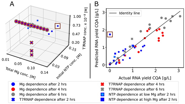
The aim is then to check if parameters to the proposed model can be found that give a good fit to the data. Although the process of model building is presented as linear, this was an iterative process of proposing different terms and fitting parameters.

Given that we are presented with an overall small set of data with a disproportionately large proportion of the data set describing RNA yield dependence on Mg concentration, the challenge consisted in proposing model terms that were able to capture the overall trends of the optimum in Mg and NTP dependence without overfitting.

The presented Model section was found to be the ‘simplest’ model to capture most non-linearities (apart from NTP dependence at high Mg as discussed in later sections).

Since the model was already overparameterised and the parameters highly correlated as is, suggesting further terms would only overfit the model. On the contrary, alpha was set to 1, as the alpha term would be inversely correlated to k_app and K₁. No enzyme degradation was assumed for now as the response of ‘levelling off’ of RNA yield was indistinguishable from the effect of K₁ and K₂. Furthermore, the degradation reaction orders n_ac, n_ba, n_Mg and n_RNA were all set to one for now.

Parameter estimation and modelling results

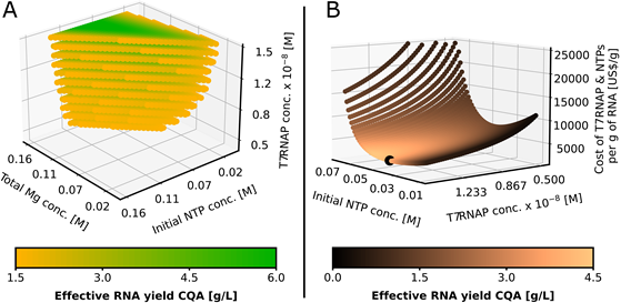
Design Space Results and Cost Analysis

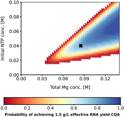
Probabilistic Design Space

Future Work

In future QbD iterations, Model-Based DoE has to be performed to investigate if the addition of other terms of physical phenomena would lead to improvements. Potential terms to be investigated include:

1. ‘Enzyme poisoning’ terms in the denominator of V_tr: K₃ [MgNTP]² and K₄ [Mg]²
2. Parameter estimation of n_ac, n_ba, n_Mg and n_RNA
3. Mg₂PPi precipitation term

However, for now, as the parameters are highly correlated, more physical, mechanistic knowledge is needed to either fix some of these parameters or constrain their bounds in parameter estimation for effective model discrimination which for the time being is not possible.

For concrete suggestions for future experiments,finding a way to measure the following physical quantities would be very helpful in model construction:

• Track the dynamic evolution of free solution NTP through in- or online measurements to narrow down the uncertainty on k_app which is the only parameter pushing the reaction forward.
• Measure the amount of Mg₂PPi precipitated to determine if V_precip should be included
• A way to measure how much RNA has degraded i.e. a way to distinguish between V_tr and V_deg